GaFT Toolbox
Example of Typical Estimation Experiment Setup
The following example will present the way the estimation experiment is specified by means of the GaFT toolbox. The example will describe a problem of estimating the state and parameter of one dimensional linear Gaussian system with one unknown parameter. It is a nonlinear estimation problem since the system is from estimation point of view bilinear. This stem from the fact that for the purpose of the estimation the unknown parameter augments the original state of the system.
Experiment setup employing GaFT
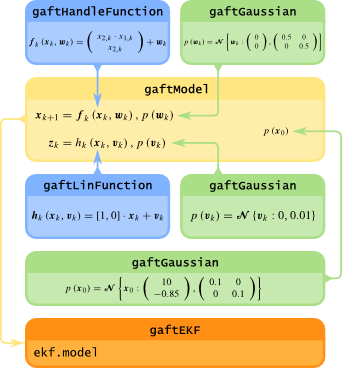
Every aspect of the estimation experiment is described using instances of toolbox classes designated for this purpose. The following picture represents all the basic objects (i.e. classes instances) necessary for the experiment setup.
Lets first describe the function defining the system dynamics. The function fk is represented as an instance of the class gaftHandleFunction which essentially employs the MATLAB® handle function. The constructor requires the transient function and the dimensions to be specified. However, due to the intend use of extended Kalman Filter (EKF) the first derivatives of the transient function to noise and state are needed as well.
As the measurement is linear, an instance of the gaftLinFunction is sufficient.
In order to complete the system description, the probability density function of all the state and measurement noises and of the prior have to be described. All three probability density functions are Gaussian hence the gaftGaussian constructor is used in the following manner.
At this point it is possible to finalize description of the system model using the constructor of the class gaftModel that uses the prepared functions and random variables description. In case that it is necessary to prepare experiment data it is possible to call the method simulate of the object model.
The final step is to setup the estimator and proceed with the estimation experiment itself. As the chosen estimator is EKF the class gaftKalman instance will be used. This class implements both the standard Kalman filter and EKF with Joseph form implementation of the algorithm. First the class constructor is called and the object method estimate is used for the estimation process.
Example of multiple estimators performance comparison
The following code will present the case when the user needs to compare results from multiple estimators. All the estimator objects can be grouped into cell array for simplicity.
The filtering estimates are finally computed for all prepared estimators employing the method estimate. Since the output of the method estimate are cell array of Gaussian probability density functions represented a object of the class gaftGaussian, it is necessary to extract the means and variances for further data analysis.
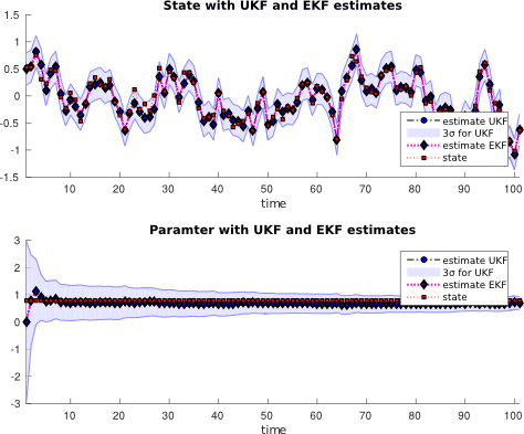
Typical results provided by the described example can be finaly processed to following graphs.


